Introduction¶

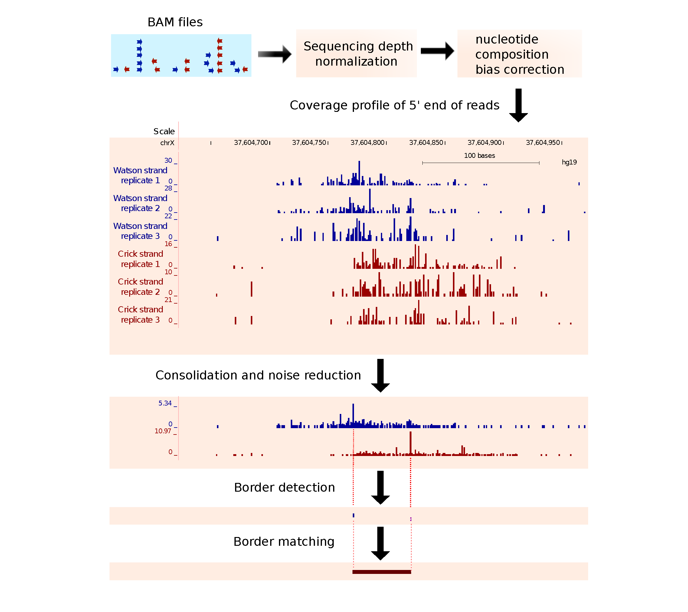
ChIP-exo allows for precise mapping of protein-DNA interactions. It uses λ phage exonuclease to digest the 5’ end of protein-unbound DNA fragments and thereby creates a homogenous 5’ end at a fixed distance from the protein binding location. After sequencing and aligning reads to the reference genome, the 5′ ends of reads align primarily at two genomic locations corresponding to two borders of protein binding site. (Rhee & Pugh, 2011 Cell; Rhee & Pugh, 2011 Nature; Mendenhall & Bernstein, 2012 Genome Biol.)

MACE is a bioinformatics tool dedicated to analyze ChIP-exo data. It operates in 4 major steps::

Sequencing depth normalization and nucleotide composition bias correction.
Signal consolidation and noise reduction using Shannon’s entropy.
Single base resolution border detection using Chebyshev Inequality.
Border matching using Gale-Shapley’s stable matching algorithm.

Release notes¶

MACE (v1.2) released on April 15, 2015.

add option (-m) to preprocessor.py let users choose the consolidation method.

EM: Entropy weighted mean (default and recommend)

AM: Arithmetic mean

GM: Geometric mean

SNR: Signal-to-noise ratio (i.e., the ratio of mean to standard deviation)

Download¶

MACE-1.2.tar.gz

MACE-1.1.tar.gz

Installation¶

Prerequisite:

gcc
python2.7
numpy
GNU Scientific Library (GSL) following the instructions.
Mac OS X users need to download and install Xcode.

Procedure to install MACE (Linux & MacOS X):

tar zxf MACE-VERSION.tar.gz

cd MACE-VERSION

#Install MACE. type 'python setup.py --help' to see install options. Note: python2.7 is needed.
python setup.py install

#Add MACE modules to python module searching path($PYTHONPATH). This step is unnecessary if MACE was installed to default location.
export PYTHONPATH=/home/user/MACE/usr/local/lib/python2.7/site-packages:$PYTHONPATH

#Add MACE scripts to Shell searching path ($PATH). This step is unnecessary if MACE was installed to default location.
export PATH=/home/user/MACE/usr/local/bin:$PATH

Walkthrough example using Frank Pugh’s CTCF ChIP-exo data¶

Please skip Step1 and Step2 if you choose to use our alignment files.

Step1: Download raw sequence data¶

Download CTCF ChIP-exo data (Accession number SRA044886) published in Cell, 2011.

wget ftp://ftp.sra.ebi.ac.uk/vol1/fastq/SRR346/SRR346401/SRR346401.fastq.gz
wget ftp://ftp.sra.ebi.ac.uk/vol1/fastq/SRR346/SRR346402/SRR346402.fastq.gz
wget ftp://ftp.sra.ebi.ac.uk/vol1/fastq/SRR346/SRR346403/SRR346403.fastq.gz

Step2: Align reads to reference genome¶

Mapping reads to reference genome. In this example, we use Bowtie to align reads to human reference genome (GRCh37/hg19). Please note Pugh’s CTCF ChIP-exo data was sequenced using SOLiD genome sequencer, so we need the color space human genome index files. Bowtie prebuild these files for download (color space genome index files). Any aligner is fine, as long as it can generate BAM or SAM format alignments file:

bowtie -S -C -q -m 1 PATH/bowtie/indexes/colorspace/hg19c SRR346401.fastq CTCF_replicate1.sam
bowtie -S -C -q -m 1 PATH/bowtie/indexes/colorspace/hg19c SRR346402.fastq CTCF_replicate2.sam
bowtie -S -C -q -m 1 PATH/bowtie/indexes/colorspace/hg19c SRR346403.fastq CTCF_replicate3.sam

Convert SAM into BAM format, then sort and index BAM files using samtools. You only need the index step if the aligner you used already produced sorted BAM file:

samtools view -bS CTCF_replicate1.sam > CTCF_replicate1.bam
samtools sort  CTCF_replicate1.bam  CTCF_replicate1.sorted
samtools index CTCF_replicate1.sorted.bam

samtools view -bS CTCF_replicate2.sam > CTCF_replicate2.bam
samtools sort  CTCF_replicate2.bam  CTCF_replicate2.sorted
samtools index CTCF_replicate2.sorted.bam

samtools view -bS CTCF_replicate3.sam > CTCF_replicate3.bam
samtools sort  CTCF_replicate3.bam  CTCF_replicate3.sorted
samtools index CTCF_replicate3.sorted.bam

You can download our sorted and indexed BAM files (Skip Step1, Step2):

wget http://dldcc-web.brc.bcm.edu/lilab/MACE/bam/CTCF_replicate1.sorted.bam
wget http://dldcc-web.brc.bcm.edu/lilab/MACE/bam/CTCF_replicate1.sorted.bam.bai
wget http://dldcc-web.brc.bcm.edu/lilab/MACE/bam/CTCF_replicate2.sorted.bam
wget http://dldcc-web.brc.bcm.edu/lilab/MACE/bam/CTCF_replicate2.sorted.bam.bai
wget http://dldcc-web.brc.bcm.edu/lilab/MACE/bam/CTCF_replicate3.sorted.bam
wget http://dldcc-web.brc.bcm.edu/lilab/MACE/bam/CTCF_replicate3.sorted.bam.bai

Step3: Preproprocessing includes sequencing depth normalization, nucleotide composition bias correction, signal consolidation and noise reduction¶

Replicate BAM files are separated by ‘,’. Reads mapped to forward and reverse strand will define two boundaries of binding sites, so finally two wiggle format files will be produced. wiggle files will be converted into bigwig format automatically if ‘WigToBigWig‘ executable can be found in your system $PATH, otherwise you need to convert them manually.:

preprocessor.py -i CTCF_replicate1.sorted.bam,CTCF_replicate2.sorted.bam,CTCF_replicate3.sorted.bam -r hg19.chrom.sizes -o CTCF_MACE

Convert wiggle into bigwig format manually. You need to download WigToBigWig program from UCSC.:

wigToBigWig CTCF_hg19_Forward.wig hg19.chrom.sizes  CTCF_MACE_Forward.bw
wigToBigWig CTCF_hg19_Reverse.wig hg19.chrom.sizes  CTCF_MACE_Reverse.bw

You can download our bigwig files directly (Skip Step3):

wget http://dldcc-web.brc.bcm.edu/lilab/MACE/bigfile/CTCF_MACE_Forward.bw
wget http://dldcc-web.brc.bcm.edu/lilab/MACE/bigfile/CTCF_MACE_Reverse.bw

Step4: Border detection and border pairing¶

Run mace.py to perform ChIP-Exo “border peak” calling and “border pairing” from two BigWig files:

mace.py -s hg19.chrom.sizes -f CTCF_MACE_Forward.bw -r CTCF_MACE_Reverse.bw -o CTCF_MACE

border pairs will be saved in file prefix.border_pair.bed (chrom, start (0-based, exclusive), end (1-based, inclusive), label, pvalue). SFB = broder pairs derived from Single Forward Border, SRB = border pair derived from Single Reverse Border, GSB, Gale-Sharpley paired Border. Below is an example

chr1    104966  104993  SFB     0.048907955391
chr1    521563  521602  SFB     0.0305608536849
chr1    714165  714215  SRB     0.018255126205
chr1    793499  793565  SRB     0.0121099793964
chr1    840126  840167  GSB     0.00494958418067
chr1    873592  873668  GSB     0.00159503506178
chr1    886925  886980  GSB     0.00402015835584
chr1    919668  919696  GSB     0.00292883762243
chr1    919680  919751  GSB     0.00791031727722
chr1    937367  937412  SFB     0.0306385665784
...

mace.py produces these files:

prefix.border.bed: This file contains single border (1nt resolution) whose coverage signal is significantly higher than local background level. Intermediate result.

prefix.border_cluster.bed: Single borders are clustered together. Each cluster might represent a single binding event. Intermediate result.

prefix.border_pair_elite.bed: high quality border pairs used to build model and estimate optimal border pair size. Intermediate result.

prefix.border_pair.bed: this file contains all detected border pairs. Final result.

Step5: visualize results using UCSC genome browser ¶

Copy the following lines and pasted into UCSC. Note the Assembly version is hg19. You need to convert peak and peak_pair files into BigBed.:

#MACE border pair and predicted motif
track type=bigBed name="CTCF MACE Border Pairs" visibility=2 color=0,0,255 windowingFunction=maximum db=hg19 bigDataUrl=http://dldcc-web.brc.bcm.edu/lilab/MACE/bigfile/CTCF_MACE_borderPair.bb
track type=bigBed name="CTCF FIMO Motif" visibility=2 color=255,0,0  windowingFunction=maximum db=hg19 bigDataUrl=http://dldcc-web.brc.bcm.edu/lilab/MACE/bigfile/CTCF_FIMO_motif.bb

#MACE consolidated signal
track type=bigWig name="CTCF MACE Forward Signal" visibility=2 color=0,0,102  windowingFunction=maximum db=hg19 bigDataUrl=http://dldcc-web.brc.bcm.edu/lilab/MACE/bigfile/CTCF_MACE_Forward.bw
track type=bigWig name="CTCF MACE Reverse Signal" visibility=2 color=102,0,0  windowingFunction=maximum db=hg19 bigDataUrl=http://dldcc-web.brc.bcm.edu/lilab/MACE/bigfile/CTCF_MACE_Reverse.bw

#Raw signals
track type=bigWig name="CTCF Raw Signal (rep1 Forward) " visibility=2 color=0,0,153  windowingFunction=maximum db=hg19 bigDataUrl=http://dldcc-web.brc.bcm.edu/lilab/MACE/bigfile/CTCF_raw_rep1_Forward.bw
track type=bigWig name="CTCF Raw Signal (rep1 Reverse) " visibility=2 color=153,0,0  windowingFunction=maximum db=hg19 bigDataUrl=http://dldcc-web.brc.bcm.edu/lilab/MACE/bigfile/CTCF_raw_rep1_Reverse.bw
track type=bigWig name="CTCF Raw Signal (rep2 Forward) " visibility=2 color=0,0,153  windowingFunction=maximum db=hg19 bigDataUrl=http://dldcc-web.brc.bcm.edu/lilab/MACE/bigfile/CTCF_raw_rep2_Forward.bw
track type=bigWig name="CTCF Raw Signal (rep2 Reverse) " visibility=2 color=153,0,0  windowingFunction=maximum db=hg19 bigDataUrl=http://dldcc-web.brc.bcm.edu/lilab/MACE/bigfile/CTCF_raw_rep2_Reverse.bw
track type=bigWig name="CTCF Raw Signal (rep3 Forward) " visibility=2 color=0,0,153  windowingFunction=maximum db=hg19 bigDataUrl=http://dldcc-web.brc.bcm.edu/lilab/MACE/bigfile/CTCF_raw_rep3_Forward.bw
track type=bigWig name="CTCF Raw Signal (rep3 Reverse) " visibility=2 color=153,0,0  windowingFunction=maximum db=hg19 bigDataUrl=http://dldcc-web.brc.bcm.edu/lilab/MACE/bigfile/CTCF_raw_rep3_Reverse.bw

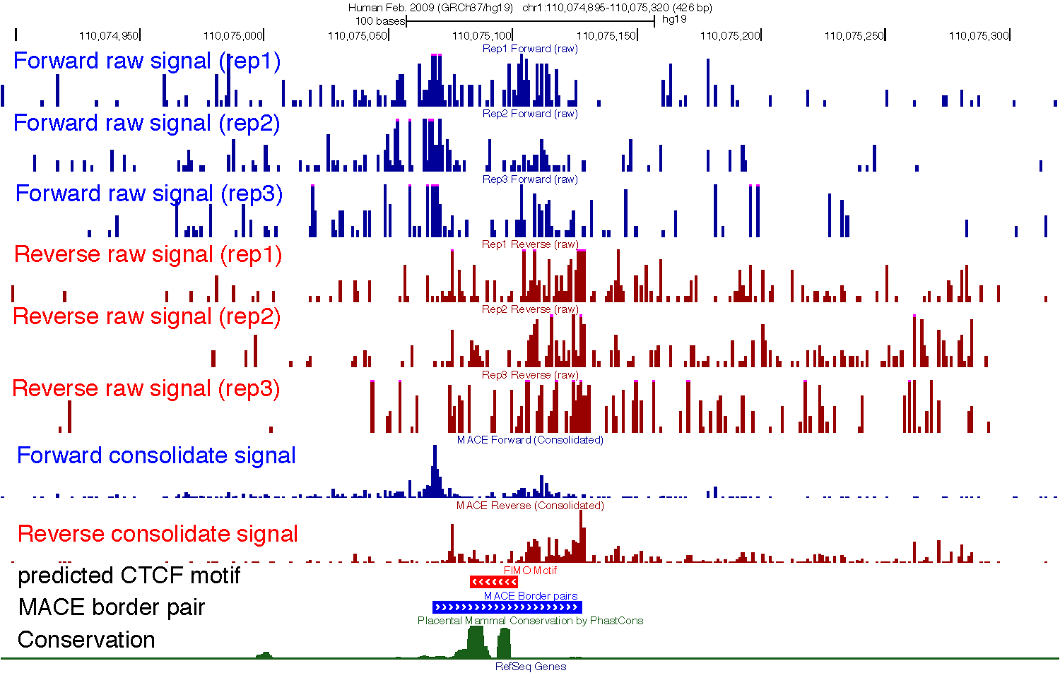
One binding site of CTCF as an example¶

An example shows border pair detection and denoising effect. Total 11 tracks were displayed in UCSC genome browser. From top to bottom, [1] - [3] forward strand coverage of three biological replicates; [4] - [6)] reverse strand coverage of three biological replicates; [7] Forward coverage signal consolidated from track [1] - [3]; [8] Reverse coverage signal consolidated from track [4] – [6]; [9] in silico predicted CTCF motif; [10] peak pairs called by MACE; [11] phastCon conservation score in mammals.

Usage¶

preprocessor.py takes BAM files as input. Consolidate the signals and output signals in wig/bigwig format.

preprocessor.py¶

Options:

`--version`	show program’s version number and exit
`-h, --help`	show this help message and exit
`-i INPUT_FILE, --inputFile=INPUT_FILE`
	Input file in BAM format. BAM file must be sorted and indexed using samTools. Replicates separated by comma(‘,’) e.g. “-i rep1.bam,rep2.bam,rep3.bam”
`-r CHROMSIZE, --chromSize=CHROMSIZE`
	Chromosome size file. Tab or space separated text file with 2 columns: first column is chromosome name, second column is size of the chromosome.
`-o OUTPUT_PREFIX, --outPrefix=OUTPUT_PREFIX`
	Prefix of output wig files(s). “Prefix_Forward.wig” and “Prefix_Reverse.wig” will be generated
`-w WORD_SIZE, --kmerSize=WORD_SIZE`
	Kmer size [6,12] to correct nucleotide composition bias. kmerSize < 0.5*read_lenght. larger KmerSize might make program slower. Set kmerSize = 0 to turn off nucleotide compsition bias correction. default=6
`-b BIN, --bin=BIN`
	Chromosome chunk size. Each chomosome will be cut into small chunks of this size. Decrease chunk size will save more RAM. default=100000 (bp)
`-d REFREADN, --depth=REFREADN`
	Reference reads count (default = 10 million). Sequencing depth will be normailzed to this number, so that wig files are comparable between replicates.
`-q QUAL_CUT, --qCut=QUAL_CUT`
	phred scaled mapping quality threshhold to determine “uniqueness” of alignments. default=30
`-m NORM_METHOD, --method=NORM_METHOD`
	methods (“EM”, “AM”, “GM”, or “SNR”) used to consolidate replicates and reduce noise. “EM” = Entropy weighted mean, “AM”=Arithmetic mean, “GM”=Geometric mean, “SNR”=Signal-to-noise ratio. default=EM

mace.py¶

mace.py first compares the signal at each nucleotide position to its background (specified by “-w”). If the signal at a position is significantly (determined by “-p”) higher than its background, MACE consider this position as “candidate border”. For most TF binding sites, we would detect multiple left borders and multiple right borders. Assume we have detected m left borders and n right borders, we have m x n border pairs in total. In theory, there is only real border pair at each TF binding site, it’s difficult to pick out this real one, but we can rank all these border pairs. The rank of each border pair is determined by two factors: signals of the two borders and the distance between the two borders. The higher the signal, the more likely the two borders are real. But only consider the signal is unfair, because other confounding factors (such as GC content, DNA sequence complexity, sequencing bias) could also affect the coverage signal. We also need to consider the size of the border pair (i.e. the genome distance between two borders), if the size of a particular border pair is much larger (or smaller) than the real TF-DNA binding size, this border pair is less likely to be real. We don’t know the real TF-DNA binding size in advance, but if we assume the TF-DNA binding size is constant across the entire genome, we could estimate it using a subset of border pairs that we called elite border pairs. In these elite border pairs, the left and right border are so prominent that we can pair them without ambiguity. The criterion to select elite border pairs is specified by “-n”. If “-n 2” was specified, we asked the signal of elite border must be at least 2 fold higher than its background.

Options:

`--version`	show program’s version number and exit
`-h, --help`	show this help message and exit
`-f FORWARD_BW, --forward=FORWARD_BW`
	BigWig format file containing coverage calcualted from reads mapped to forward strand.
`-r REVERSE_BW, --reverse=REVERSE_BW`
	BigWig format file containing coverage calcualted from reads mapped to reverse strand.
`-s CHROMSIZE, --chromSize=CHROMSIZE`
	Chromosome size file. Tab or space separated text file with 2 columns: first column contains chromosome name, second column contains chromosome size. Example:chr1 249250621 <NewLine> chr2 243199373 <NewLine> chr3 198022430 <NewLine> ...
`-o OUTPUT_PREFIX, --out-prefix=OUTPUT_PREFIX`
	Prefix of output files. NOTE: if ‘prefix.border.bed’ exists and was non-empty, peak calling step will be skipped! So if you want to rerun mace.py from scratch, use different ‘prefix’ or delete old ‘prefix.border.bed’ before starting.
`-p PVALUE_CUTOFF, --pvalue=PVALUE_CUTOFF`
	Pvalue cutoff for border detection and subsequent border pairing. default=0.05
`-m MAX_DISTANCE, --max-dist=MAX_DISTANCE`
	Maximum distance allowed for border pairing. default=100 (bp)
`-e FUZZY_SIZE, --fz-window=FUZZY_SIZE`
	Peaks (i.e. borders) located closely within this window will be merged. default=5 (bp)
`-w WINDOW_SIZE, --bg-window=WINDOW_SIZE`
	Background window size used to determine background signal level. default=100 (bp)
`-n SIGNAL_FOLD, --fold=SIGNAL_FOLD`
	Minmum coverage signal used to build model (i.e. estimate optimal peak pair size). default=2.0

Comparing 4 consolidation methods¶

Consolidation is the process of combining signals from replicates together. To make the real TF binding boundaries prominent, we hope this process could also boost signal at real TF-DNA boundaries and reduce noise signals (see CTCF example above).

We provide 4 different methods to consolidate signals:

EM: Entropy weighted mean (default and recommend)
AM: Arithmetic mean
GM: Geometric mean
SNR: Signal-to-noise ratio (i.e., the ratio of mean to standard deviation)

As shown in the table below, AM is not a good choice because it’s sensitive to outlier(s). Due to the over dispersion of count data, SNR is also not a good choice. “GM” and “EM” are very close, but GM is sensitive to missing values.

Caveats¶

MACE is designed to process ChIP-exo data whose quality is reasonably good. According to ChIP-exo procedure, coverage signals at protein binding boundaries should be significantly higher than background. If MACE fails to build the model, this usually indcates either the experiment was not successful or the IP target protein is very dynamic thus does not have fixed binding boundaries. In this situation, ChIP-exo is basically downgraded to ChIP-seq and should be processed using ChIP-seq method (such as MACS) accordingly.

Reference¶

Wang, L., Chen, J., Wang, C., Uusküla-Reimand, L., Chen, K., Medina-Rivera, A., et al. (2014). MACE: model based analysis of ChIP-exo. Nucleic Acids Research. doi:10.1093/nar/gku846

Contacts¶

Wang, Liguo <wang.liguo@mayo.edu>
Kocher, Jean-Pierre A. <kocher.jeanpierre@mayo.edu>
Li, Wei <wl1@bcm.edu>

Introduction¶

Release notes¶

Download¶

Installation¶

Walkthrough example using Frank Pugh’s CTCF ChIP-exo data¶

Step1: Download raw sequence data¶

Step2: Align reads to reference genome¶

Step3: Preproprocessing includes sequencing depth normalization, nucleotide composition bias correction, signal consolidation and noise reduction¶

Step4: Border detection and border pairing¶

Step5: visualize results using UCSC genome browser ¶

One binding site of CTCF as an example¶

Usage¶

preprocessor.py¶

mace.py¶

Comparing 4 consolidation methods¶

Caveats¶

Reference¶

Contacts¶

Table Of Contents

This Page

Navigation

Introduction¶

Release notes¶

Download¶

Installation¶

Walkthrough example using Frank Pugh’s CTCF ChIP-exo data¶

Step1: Download raw sequence data¶

Step2: Align reads to reference genome¶

Step3: Preproprocessing includes sequencing depth normalization, nucleotide composition bias correction, signal consolidation and noise reduction¶

Step4: Border detection and border pairing¶

Step5: visualize results using UCSC genome browser¶

One binding site of CTCF as an example¶

Usage¶

preprocessor.py¶

mace.py¶

Comparing 4 consolidation methods¶

Caveats¶

Reference¶

Contacts¶

Table Of Contents

This Page

Quick search

Navigation

Step5: visualize results using UCSC genome browser ¶